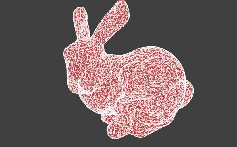
Lets say you have mesh data in the typical format, triangulated, vertex buffer and index buffer. E. g. something like
>>> vertices

[[[ 46.27500153  19.2329998   48.5       ]]

 [[  7.12050009  15.28199959  59.59049988]]

 [[ 32.70849991  29.56100082  45.72949982]]

 ...,

>>> indices

[[1068 1646 1577]
 [1057  908  938]
 [ 420 1175  237]
 ...,
Typically you would need to feed it into OpenGL to get an image out of it. However, there are occasions when setting up OpenGL would be too much hassle or when you deliberately want to render on the CPU.
In this case we can use the OpenCV to do the rendering in two function calls as:
img = np.full((720, 1280, 3), 64, dtype=np.uint8)

pts2d = cv2.projectPoints(vertices, rot, trans, K, None)[0].astype(int)
cv2.polylines(img, pts2d[indices], True, (255, 255, 255), 1, cv2.LINE_AA)See the documentation of cv2.projectPoints for the meaning of the parameters.
Note how we only project each vertex once and only apply the mesh topology afterwards. Here, we just use the numpy advanced indexing as pts2d[indices] to perform the expansion.
This is pretty fast too. The code above only takes about 9ms on my machine.
In case you want filled polygons, this is pretty easy as well
for face in indices:
cv2.fillConvexPoly(img, pts2d[face], (64, 64, 192))However, as we need to a python loop in this case and also have quite some overdraw, it is considerable slower at 20ms.
Of course you can also combine both to get an image like in the post title.
From here on you can continue to go crazy and compute face normals to do culling and shading.
